Selected Screenshots

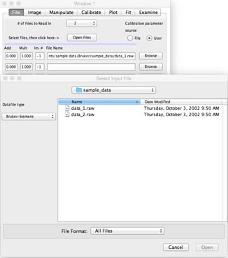
Home Download Get Key Technical Details Screen Shots FAQ XRD Basics About Us Privacy/Security	File Input Panel
	We are reading in two data files. We have already selected one called "data1.raw" with a multiplicative value of +1 and are in the process of selecting a second background scan called "data2" with a multiplicative value of +1. After selecting the files we want, we will click on the "Open Files" button to actually read them in.

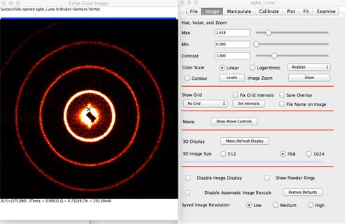
Image Panel
The data have been read in but not yet calibrated (e.g., the beam center position is not set). We are setting an appropriate color scale.
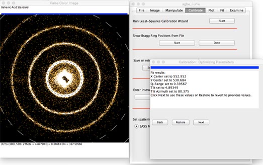
Calibrate Panel
We can calibrate the instrument parameters (effective angular range of the detector, center of the pattern) by measuring a calibration standard and comparing it to known d-spacings. The dashed circles correspond to positions where we ought to see Bragg rings for the material. When we are done the circles will be centered on, and have the same diameter as, the experimental data.
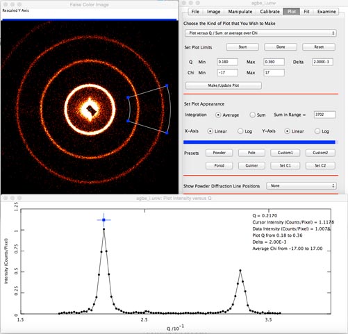
Plot Panel
We are making a radial plot of the intensity, using the data inside the region defined by the wedge. We can set the corners of the wedge with the mouse or by typing into boxes on the right. The actual plot appears at the bottom. We can drag the cursor around to find out the X and Y values at any point in the image.
Least-squares Fit
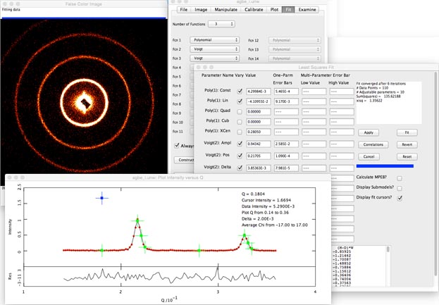
We have done a least-squares fit to the data, taking as our model a constant plus two Voigt lineshapes. The data points are now shown in red, the fitted function as a black curve, and the residual appears below.
Examine Panel
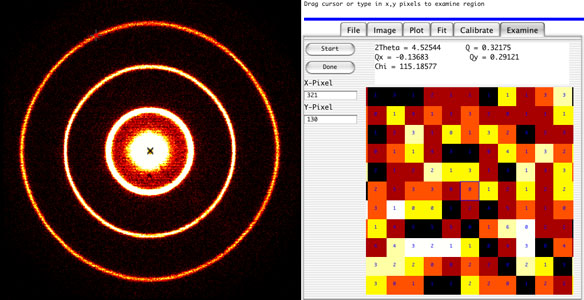
We can drag a cursor to a region of interest, or input its X and Y coordinates, and examine the data pixel by pixel.
Info Window
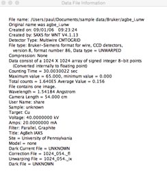
Depending on the data file file format, information on the same and data collection conditions may be available from the file header. In any case we can get statistical information such as maximum and minimum intensity, etc.
Statistics Window
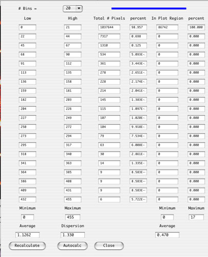
We have calculated histogram information on how many pixels are in different intensity ranges.
Help Panel
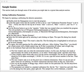
Onboard help is available in the form of a hyperlinked file with detailed information on each feature and a short tutorial section.
Grid Overlay
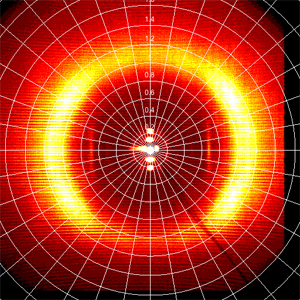
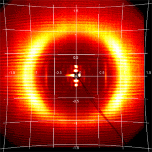
For data with some structure, such as this fiber diffraction pattern, it may be useful to overlay a grid in polar or Cartesian coordinates.
Wide Angle Diffraction
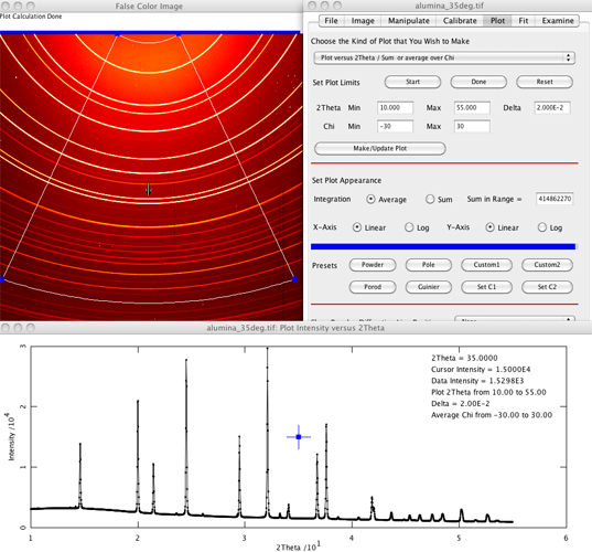
For this alumina diffraction pattern the detector was rotated 35 degrees away from the main beam.
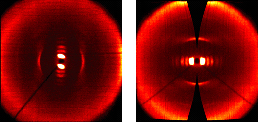
Fraser Fiber Correction
The left hand image shows the raw fiber diffraction pattern. The fiber axis is approximately horizontal, so 00L reflections are along a horizontal axis and HK0 reflections along a vertical axis. The right hand image shows the image after the Fraser correction has been applied. Data are now on a true Cartesian qx-qy grid. The horizontal axis lies along the equator (HK0 reflections) and the vertical axis lies along the meridian. The dark arc is due to areas that are geometrically inaccessible due to the curvature of the Ewald sphere. The pattern is symmetric under reflection about a vertical axis but not necessarily about a horizontal axis.

Last updated September 4, 2023